2020年5月19日

Thingworx Analytics Introduction 3/3: Time Series Data TTF Prediction


This is the 3rd article of series: Thingworx Analytics introduction.
1st article introduces Analytics Function and Modules.
2nd article introduces Non Time Series TTF prediction.

Environment: Thingworx Platform 8.5, Analytics Server 8.5, Analytics Extension 8.5.

In TTF prediction, Time Series Data model is better than Non Time Series Data model.
What’s Time Series Data model?
As per Machine Learning concept, the process of training model is to find the best matching parameters, and to use them to combine with features to calculate the result values.
For Non Time Series Data models, it’s not relevant between current values and previous values.
But for Time Series Data, during each time of calculation, it will check not only current values, but also previous values, and the previous values are time relevant.
There’re 2 important terms here: look back size, and data sampling frequency.
Look back size = numbers of data samples need to look back.
Data sampling frequency = the frequency of taking a new data sample.
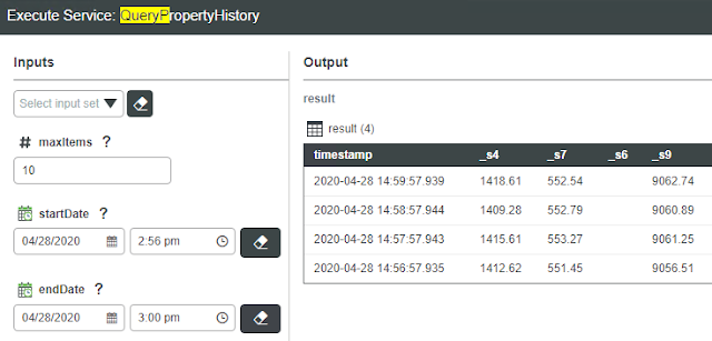
Look back size * Data sampling frequency = the total numbers will be feed to run calculation, for which I call it Look back area, the data is queried from Value Stream, with maxItems = look back size, and startDate = current date – look back area.
For example, if look back size = 4, data sampling frequency = 1 minute, then look back area = 4 minutes.
Thingworx used Value Stream to log Time Series Data, we can run service of QueryProperyHistory to get historic data:


Some other notes for TTF prediction models:
• Always set useRedundancyFilter = true
• Always set useGoalHistory = false
• Always set lookahead = 1
• Training time is much longer than Non Time Series data

After the model is published, test of model requires to input not only current values of all features, but also previous values as defined in look back size, than click Add Row to add the new record.
When creating Analysis Events, please be noted that the Thing Properties of Inputs Mapping should be Logged, because only Logged Properties can be queried with historic values from Value Stream.
And for Results Mapping, if we bind the result to Thing Property, even if that Property is set Logged, somehow the update by Analytics will not be logged into Value Stream. We can create another Property, and bind it with Results Mapping, and sync it with the final Property you’re monitoring by Service or Subscription, and Log it into Value Stream. After that, we can track all of the historic changes with TimeSeriesChart.
Below charts show the comparison between Time Series Data models predicted TTFs and actual TTFs.


We can see that, compare to Non Time Series models, the prediction is much more accurate, and is faster to match the actual TTF curve.
Below table lists out the settings of all models:


Another note, to make sure to write all features into Value Stream in same moment in same record, we should use UpdatePropertyValues instead of SetPropertyValues.
Some codes for reference:
----------------------------------------------------------------------
// Use UpdatePropertyValues to make sure to update all attribute in the same moment

var params = {
    infoTableName : "InfoTable",
    dataShapeName : "NamedVTQ"
};

// CreateInfoTableFromDataShape(infoTableName:STRING("InfoTable"), dataShapeName:STRING):INFOTABLE(VSTestDataShape)
var tempDable = Resources["InfoTableFunctions"].CreateInfoTableFromDataShape(params);

var time = new Date();
tempDable.AddRow({
       time: time,
    name: "F1",
    quality: "GOOD",
    value: 71
});

tempDable.AddRow({
       time: time,
    name: "F2",
    quality: "GOOD",
    value: 72
});

tempDable.AddRow({
       time: time,
    name: "F3",
    quality: "GOOD",
    value: 73
});

tempDable.AddRow({
       time: time,
    name: "F4",
    quality: "GOOD",
    value: 74
});

tempDable.AddRow({
       time: time,
    name: "F5",
    quality: "GOOD",
    value: 75
});

me.UpdatePropertyValues({
       values: tempDable /* INFOTABLE */
});

var result = tempDable;
----------------------------------------------------------------------


2020年5月18日

Thingworx Analytics Introduction 2/3: Non Time Series TTF Prediction


This is the 2nd article of series: Thingworx Analytics introduction.
1st article introduces Analytics Function and Modules.
3rd article introduces Time Series TTF prediction.

This article is for TTF(Time to Failure) prediction, it is quite useful in IoT applications.
Environment: Thingworx Platform 8.5, Analytics Server 8.5, Analytics Extension 8.5.

Step 1, configure Analytics setting.
Click Analytics icon >> Analytics Manager >> Analysis Providers, create a new Analysis Provider, Connector = TW.AnalysisServices.AnalyticsServer.AnalyticsServerConnector.
Click Analytics Builder >> Setting, select and set Analytics Server.

Step 2, create Analysis Data.
We need to prepare a CSV format data file and a JSON format data type file.
For CSV file, its 1st line is its header, should be equivalent with definition in JSON file.
JSON file structure can refer to:
---------------------------------------------------
[
       {
              "fieldName": "s2",
              "values": null,
              "range": null,
              "dataType": "DOUBLE",
              "opType": "CONTINUOUS",
              "timeSamplingInterval": null,
              "isStatic": false
       },
       {
              "fieldName": "s3",
              "values": null,
              "range": null,
              "dataType": "DOUBLE",
              "opType": "CONTINUOUS",
              "timeSamplingInterval": null,
              "isStatic": false
       }
]
---------------------------------------------------
CSV file includes below information:
• goalField, for result checking.
• key parameters fields.
• Data filter field, e.g. we can use filed record_purpose to filter training data out of scoring data, while training data is for model training, and scoring data is for validation or test.
• If the dataset type is time series data, we need to create 2 additional fields to identify AssetID(sequence of failure) and Cycle(cycle number inside AssetID).

Here I used a public NASA dataset for training, download URL:
When data is ready, click Analytics Builder >> Data >> New..
Select CSV file and JSON file, check option of “Review uploaded metadata”.
For most parameter fields, the data type should be Continuous.
And for goal filed, data type should be Continuous or Boolean, in this example we use Continuous.
Click “Create Dataset”.
When it’s done, the newly created Data will be showed in Datasets list.
Select the data, and click Dataset >> View >> Filters >> New, to create filter.

Step 3, create Machine Learning model.
Click Analytics Builder >> Models >> New.
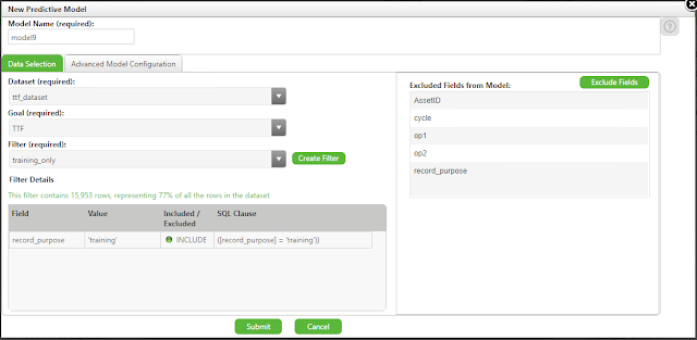
Select dataset, and select goal field and filter, and select excluded fields:


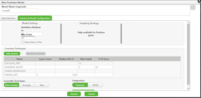
Click Advanced Model Configuration:


In Machine Learning, normally we split data into training set, validation set, and test set, with rate of 60%, 20%, 20%.
In this step, we can use Filter to filter out test data, and use Validation Holdout % to define percentage of validation, we can use default setting of 20%.
Learning Techniques includes possible Machine Learning algorithms, we can manually add algorithms and modify parameters.
For each new model, I’d suggest to training it with different algorithms, and test them to get the most accurate one.
For same algorithm, we can train it with different parameters.
Ensemble Technique is the mix method of multiple algorithms, we can try and test with different settings.
My training methods:


Click Submit to create model.
For small dataset, it requires little training time, but for time series data, it requires much longer training time.
For any dataset, the data size is bigger, the training time is longer.
When it’s done, we can find the new model in Analytics Builder >> Models.
Select the model and click View, then we can see the model information.
Select the model and click Publish, then we can publish it to Analytics Manager, we can see it in Analytics Manager >> Analytics Models, and a Test Page will pop up.

Step 4, test model.
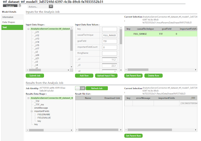
The test page will pop up when model is published, and we can also access it by: Click Analytics Manager >> Analysis Models, select model, click View >> Test:


For causalTechnique, normally we set it as FULL_RANGE.
For goalField, input name of goal field.
Then input values of all features/sensors, and click Add Row. In case of time series data, we need to add multiple rows for it.
Select 1st row, click Set Parent Row, then click Submit Job.
System will calculate and get result based on model and input values.
It might take a few seconds for calculation.
Under below Results Data Shape, select AnalyticsServerConnector.xxx, click Refresh Job, then you can see the result value.
For more detail information, you can check from Analysis Jobs.

Step 5, set automatic calculation.
After model creation, we might monitor it for some time, to check the prediction with actual values.
Take the NASA data for example, we could use some of its data for comparison, you may refer to below steps.
Firstly, build a Data Table, load CSV data into it.
Then build a Thing, create attributes mapping with model features.
Then create a Timer, to read data from Data Table and write value into Thing timely, and use these data for test.
Click Analytics Manager >> Analysis Models, enable the newly created model.
Click Analysis Events >> New, set Source Type = Thing, set Source as newly created Thing, set Event = DataChange, set Property as trigger attribute.
Save and create new Event under Analysis Events, click Map Data >> Inputs Mapping, set Source Type = Thing, and bind model features with Thing Property.
Tips: model feature names are started with _, and that causalTechnique & goalField can use static values. So if we defined such features in Thing, we can use Map All in this step, which will map all features automatically.
Then click Results Mapping, bind the test result with Thing Property. Please be noted, system generated result will be updated, but will NOT be logged into Value Stream, so we need to build another Property, and use Service to sync the data and log to Value Stream eventually.
When Event is setup, system will monitor and trigger automatically, and output value by calling internal Analytics API.
For both manual test and Event calculation, we can see the details in Analysis Jobs.
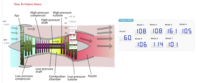
My TTF Demo Mashup for reference:


Comparison of different models:


Some notes:
• If you didn’t’ install Analytics Platform, then Analytics will run job in Synchronous mode. That means if many jobs are submitted in same time, then only 1 job will be running in that moment, and the other jobs will be pending(state=waiting). To avoid waiting jobs, we can manually create multiple trigger properties, and use PAUSE in JavaScript to delay the time in purpose.
• If raw data has many features, we can build a smaller model with 2 features, and use it to train and test, to find issues in modeling, and to optimize logic in Data Table/Thing/Timer, then extend to all features.
• Be cautious of using Timer, because wrong operations might cause mass data in Value Stream, or generate lots of Waiting Jobs. Too many Waiting Jobs will block analysis and prediction. We can use Resource of TW.AnalysisServices.JobManagementServicesAPI.DeleteJobs to delete jobs by force, and we can check Job’s total number by running Data Table’s Service of TW.AnalysisServices.AnalysisDataTable.GetDataTableEntryCounts.


Thingworx Analytics Introduction 1/3:Analytics Function and Modules


This is the first article of series: Thingworx Analytics introduction.
2nd article introduces Non Time Series TTF(Time to Failure) prediction.
3rd article introduces Time Series TTF prediction.

In year 2015, PTC acquired Machine Learning company ColdLight, and integrate its products into Thingworx, and renamed to Thingworx Analytics.
PTC Thingworx Analytics Help Site lists its functions:
• Explanatory Analytics: such as to identify a signal’s value
• Descriptive Analytics: such as calculation of average value, median value, and standard deviation value.
• Model Generation: model creation of prediction, includes some popular Machine Learning algorithm.
• Predictive Scoring: to predict result value based on trained model and parameters.
• Prescriptive Scoring: to change result values by modifying model parameters.
• Confidence Models: convert prediction result into rates of value ranges.
• Anomaly Detection: to filter out abnormal signals by comparing high and low limits.
• Time Series Predictions: some signal are time series related, so for each time of prediction, besides checking current values, it will also check the values of previous cycles.
• Learners and Ensemble Techniques: Machine Learning algorithm and mixing method.

Analytics implemented these Machine Learning algorithm:
• Linear Regression
• Logistic Regression
• Decision Tree
• Neural Network
• Random Forest
• Gradient Boost

And let’s see Analytics modules.
Analytics has 3 installation modules: Analytics Server, Analytics Platform, Analytics Client(extension).
When Analytics Server is installed, it will add these services into Windows OS:
• twas-analytics-worker-1
• twas-analytics-worker-2
• twas-analytics-worker-3
• twas-async-ms
• twas-sync-ms
• twas-twx-adapter
• twas-zookeeper

And create these entities into Thingworx platform:
• StatisticalCalculationMicroserver, with some SPC calculation services.
• StatisticalMonitoringMicroserver, with some SPC distribution services.
• Some Thing entities with AnalyticsServer in names, can be found in Monitoring >> Remote Things, it can also be accessed by Thingworx Server API.
• Data Tables with prefix of TW.AnalysisService, they’re Database of Analytics.
• Resources with prefix of TW.AnalysisService, mapping with Analytics Builder functions.

Analytics Platform is an independent module, it can improve performance, and we can run basic prediction with it.
Analytics Client can be installed as an extension, Thingworx will add an Analytics icon after installation in left action bar.
Analytics action bar has 2 categories of functions: Builder and Manager. Builder is for model building, and Manager is for background handling.

2020年5月11日

从《巫师3》看游戏作为第九艺术

这段时间陆续地玩《巫师3》,被它深深地吸引,深刻地体会到游戏作为第九艺术的魅力。
《巫师3》是角色扮演类游戏,如同美剧一样,有很强的代入感,有很多另人感动的细节。
本文从文学性、戏剧性、美术性这三个方面来分析它的艺术性。

首先是文学性。
我们知道《巫师3》是根据同名奇幻小说改编的,小说的世界观非常宏大,人物刻画也非常丰满,而游戏也保留了这个特色,比如几乎每个NPC在互动时都有相符的台词。
而主要人物的性格和情节的发展也非常匹配。
有很多玩家津津乐道于游戏丰富的啪啪啪场景(有野合、独角兽震、船震、云震等),但是如果仔细分析的话,这些场景的设计也是巧妙且合适的。
以凯拉、特莉丝、叶奈法为例。
凯拉的场景发生在沼泽,野合万物兴。凯拉是杰洛特生命中的过客,不管情节怎么发展,他们最终都不会在一起。因此两人必然只是露水姻缘,如梦似幻。而凯拉也喜欢这种自在的方式。
特莉丝的场景发生在灯塔,在城市的边缘。特莉丝刚刚被房东赶出,也刚刚逃出女巫猎人的魔爪,因此两人都是城市边缘的浪子,但是灯塔的光带给他们温暖和希望,预示着他们可以在一起。
叶奈法就不同了,两次浪漫场景都发生在室内,在她的房导间,这说明在两人的关系中,她是主导者。

再来看戏剧性。
这可以从游戏中的两场戏中戏看出一斑。
一场戏是为了引出变形怪,专门编了一出剧,主题是巫师救变形怪,而对应的现实是巫师需要变形怪的帮助。
另一出戏是普西拉在翠鸟旅店演唱Wolfen Storm。这首歌的主题是杰洛特和叶奈法的爱情故事。这是完整的一首歌,在YOUTUBE上有几十种语言的演唱版本,游戏还专门制作了完整的MV,我们可以看到听众男默女泪,有很多微表情的特写。

再来看美术性。
我的感觉是,此游戏油画感很强,非常注重光线的运用。
我们看下面这个《林中夫人》的壁挂,非常鲜明的沃特豪斯的风格:


杰洛特在迷雾之岛的小屋里找到希里,发现她已经没了呼吸,这个场景分明让人想到圣母抱着十字架下的耶稣,而此后的希里苏醒也对应着耶稣复活:


最后我们再来看特莉丝在屋里,杰洛特慢慢走进她那昏暗的、阁楼里的小屋,这里的烛光、阴影、墙上的画、墙角的静物、斑驳的墙面,这一切都让人不由地想起伦勃朗的油画,而这一切都是实时渲染形成的